Cats2D Multiphysics > Developments > Brownian motion

Semi-stochastic model of Brownian motion

The semi-stochastic model demonstrated here uses the solution to the diffusion equation as a probability distribution to randomly perturb particle velocities during path integration. Some mathematical details are found here.

This economical treatment is accurate when a good random number generator is used. The 32 bit random number generator typically provided by rand() in C/C++ produces 2^31 (2.14 billion) distinct random numbers. Apparently we should use no more than the square root of this number (about 46,000) if we want an excellently uniform distribution. This isn't enough—I routinely use millions of particles—and the initial results showed signs of a poor distribution. Satisfactory results were achieved after I added a 64 bit permuted congruential generator to Cats2D. As an added precaution, I use separate random number streams to determine the direction and size of the perturbation to avoid any correlation between these variables.

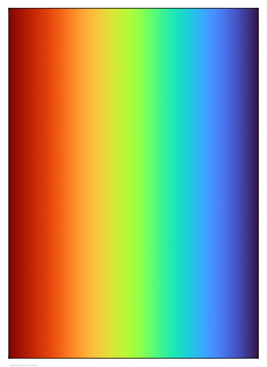
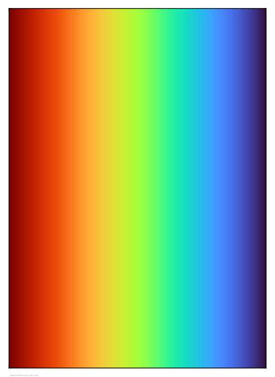
In the following tests, 1,824,459 particles are uniformly distributed in space and colored to represent a linear stratification. On the left is a plot of the particles themselves, represented by small colored dots. On the right is a color shade plot of a least squares projection of particle values onto the finite element basis functions. The images look identical, but differ greatly in how they were created.

   

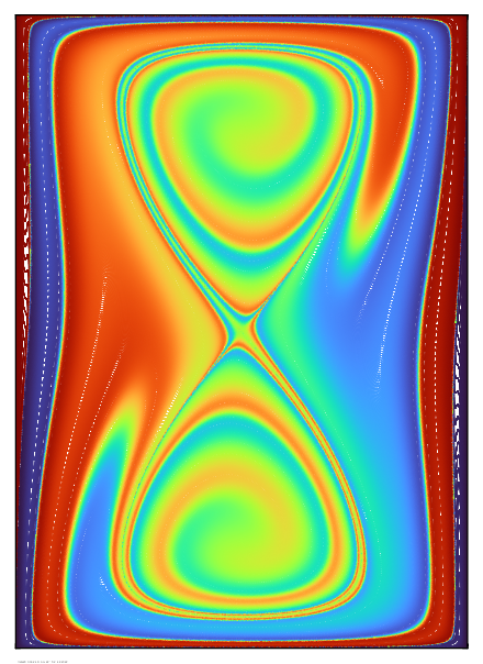
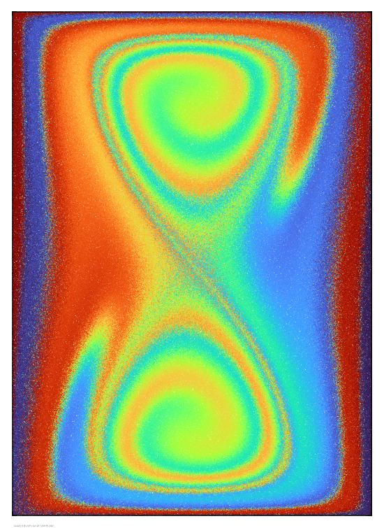
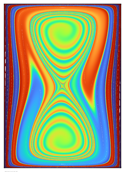
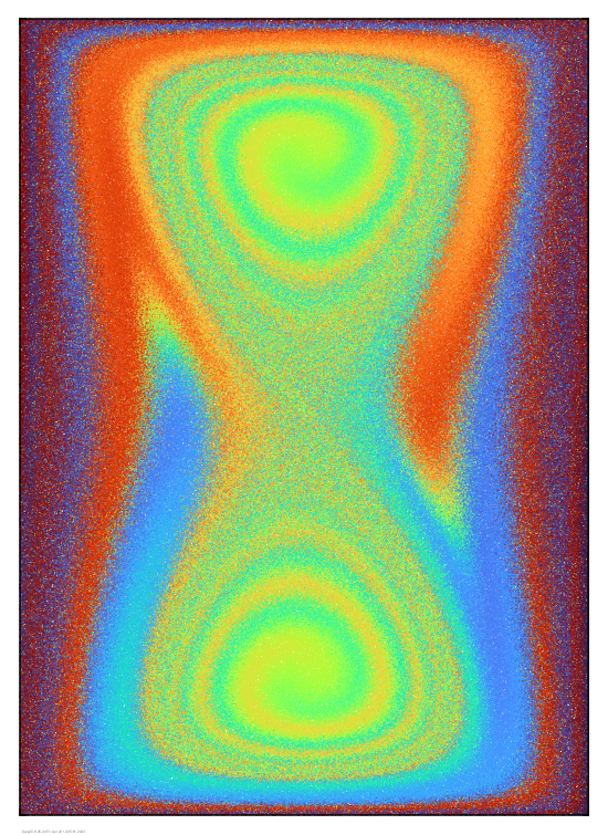
These next images show particle plots after 5 time units of mixing by a steady driven cavity flow. This flow configuration has two internal lobes of trapped fluid that do not mix with the outer flow. Mixing without Brownian motion is shown on the left, and with Brownian motion is shown on the right (equivalent to Peclet number = 10^5). The diffusive effect of Brownian motion is evident.

    

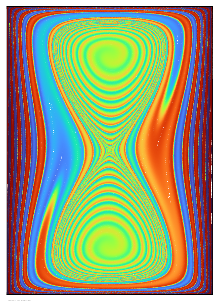
The effect is more pronounced after 10 time units, though much structure is still evident in the concentration field within different regions of the flow.

    

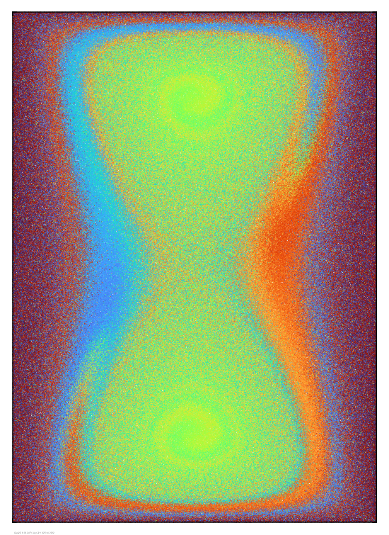
After 20 time units, concentration layers have largely disappeared within separate regions of the flow.  Large gradients persist near the separation streamline where transport occurs mostly by diffusion.

    

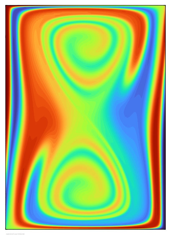
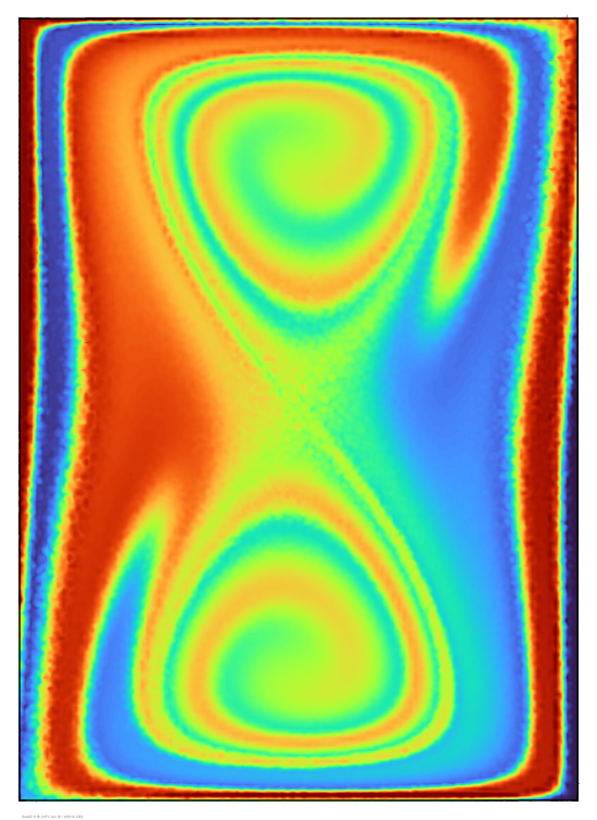
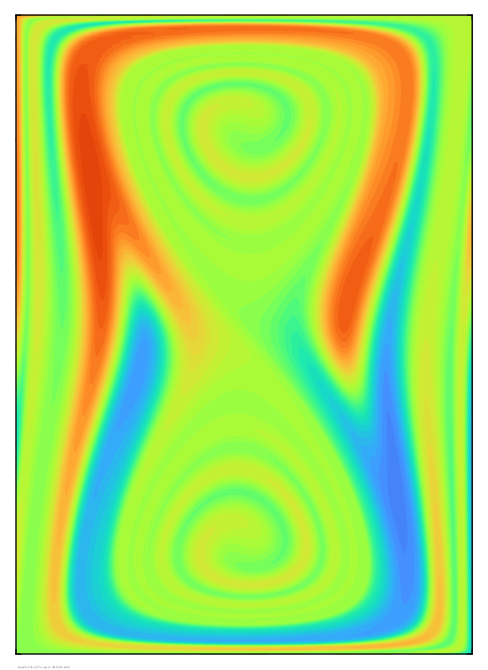
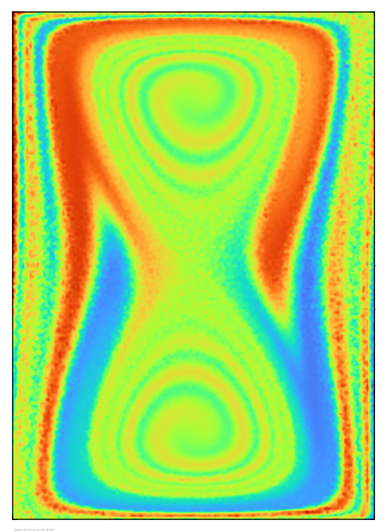
Next I show how solutions to the convective-diffusion equation at Peclet = 10^5 compare to the concentration field obtained by projecting the particle values onto a finite element basis.

After 5 time units:

   

After 10 time units:

    

After 20 time units:

    

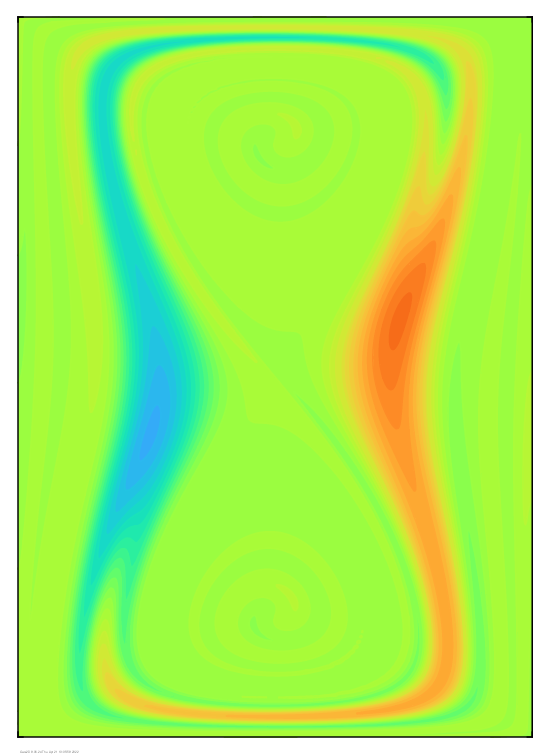
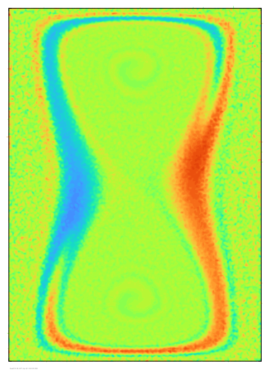
The projected field (shown on the right) is obviously noisy, but I think the results look pretty good overall.