Analyzing flow topology

Cats2D Multiphysics > Research Topics > Analyzing flow topology

Analyzing flow topology

Critical point finding for incompressible flows

In 1992 I developed a critical point finding algorithm for CFAL. There are some nice papers about this method in the documentation page of this web site. The CFAL version that I wrote used the downhill simplex method, a multi-dimensional minimization algorithm, to find the extrema of the stream function, which mark vortex centers. These are so-called critical points of the stream function, which are topological features of the flow.

An incompressible flow in two dimensions has two other types of critical points, which are separation points at boundaries, and internal stagnation points, which occur at saddle points in the stream function. These can be found by seeking minima in the velocity that are also zeroes, i.e. stagnation points. By comparing these stagnation points to the vortex centers already found, we can identify the saddle points by inference.

Once these critical points are known, we can make a nice picture of the topology of a flow showing only the critical points and critical streamlines, free of extraneous detail. Here is an example of a cavity flow with left and right ends driven in opposite directions:

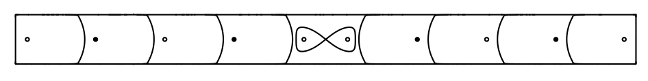
This approach is robust in the sense that it reliably finds and correctly identifies all the critical points across many orders of magnitude of velocity, on meshes both coarse and fine. The streamline values of the saddle and the vortexes it encloses are 4.2 X 10^-12 and 6.8 X 10^-12 respectively, more than ten orders of magnitude weaker than flow in the outermost vortexes. But the method is slow because the minimizations do not use any gradient information to accelerate convergence and must be repeated many times to find all the minima. We'll get to that in a minute. About now you're thinking "big deal, driven cavity blah blah, what good is this picture?" so we'll take a brief interlude to look at a critical point plot in the slot coater:

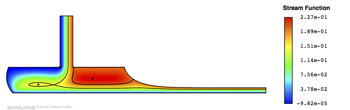
Here's the deal: without a very fine algorithm to find that interior stagnation point under the slot exit, you are likely to miss that region of trapped fluid behind the saddle. Ordinary streamline plots often fail to reveal much detail in regions of slow flow. Scriven's group studied this problem for several years without realizing this closed recirculation was present. Residence time in this region is set by the slow diffusion characteristic of liquids, and therefore is very long. This might pose problems for coating liquids that can "age" in some manner, so we would like to know of its existence.

Goodwin installed a critical point plot capability in the code, but instead of minimization he used Newton's method to directly find zeroes of the velocity field and the stream function gradient. This works great at identifying stagnation points, but terrible at finding zeroes in the stream function gradient, making it impossible to reliably determine which points are vortex centers and which are saddles.

This approach gives an unsatisfactory result because the finite element representation of the stream function has discontinuous derivatives at the element boundaries, allowing zeroes to "hide" between the elements (this is what I call a know your methods moment). Goodwin tried using the Hessian of the stream function to identify the type of critical point. This requires evaluating second derivatives of the stream function, with further degradation of accuracy. It gives the wrong answer about half the time.

To make things better, I have started with Goodwin's code to find the zeroes of the velocity field, which does so fast and reliably. Then I determine the type of critical point by applying a local patch test to the stream function around each critical point to explore whether it is an extremum or a saddle. It is important to explore neighboring elements when a critical point lies on or near an element boundary, and careful numerics are needed to detect shallow extrema in slow moving areas of the flow. A particularly demanding example is this flow in a long narrow cavity with top and bottom sides driven in opposite directions:

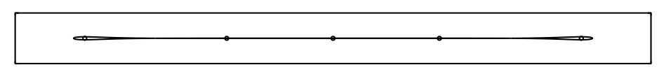
The method is quite robust, and much faster than the CFAL version I wrote 25 years ago. The difference in stream function value between the center vortex and the saddles flanking it equals 1.5 X 10^-11, ten orders of magnitude smaller than the stream function itself.

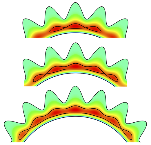
Below I show an excellent demonstration of this tool. Goodwin, bored as usual, threw together this problem at the dining room table one Saturday and sent it to me. Depicted below is the cross section of a cylinder eccentrically placed and rotating within a deeply corrugated outer wall. A fluid fills the space between them. Goodwin calls this problem Lisa Simpson's Hair. This problem makes a great demonstration of the critical point finding algorithm.

I think there are 45 critical points in Lisa Simpson's Hair. The structure of the flow is rather intriguing, too. Saddle streamlines are nested seven deep, enclosing fifteen co-rotating vortex centers. Here are the three innermost saddle streamlines, enclosing seven vortex centers:

The anatomy of a flow

Topology plots are particularly useful for visualizing complex time-dependent flows with separation. Such flows often appear inscrutable in conventional vector or streamline plots. By plotting only the saddle and separation streamlines we reveal the skeleton of the flow. This alone is useful, but combined with the bicolor scale it does much to clear away the fog.

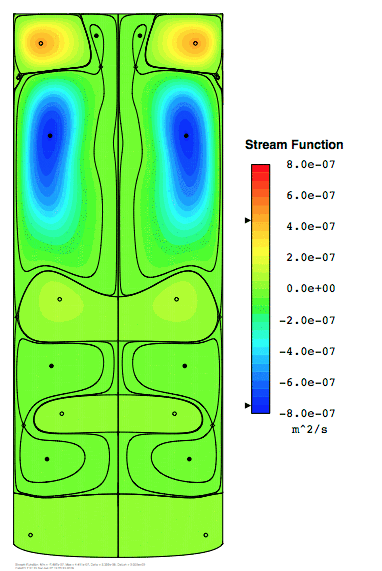
By setting the two colors to represent positive and negative values of streamfunction, we obtain a visual cue that shows whether flow is recirculating clockwise or counter-clockwise in a closed flow. Consider the unstable vertical Bridgman flow shown below, which exhibits a 12 second limit cycle. Liquid rises at the centerline and sinks at the walls in the blue regions, and vice versa in the red regions. Mouse over the images to see how these regions evolve over the course of the limit cycle. By comparison the rainbow scale is ineffective, not to mention ugly.

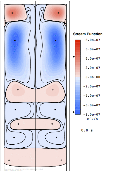
A change in hue at any given point in the flow indicates the flow direction has reversed there. Although there is a lot of intriguing action in the upper part of the melt, the region adjacent to the growth interface at the bottom remains red throughout the limit cycle, so we know that flow never reverses there. Flow reversal has significant implications for mixing along the interface, and also melting back of the interface. Its absence here suggests that growth conditions remain largely undisturbed by the limit cycle.

In contrast, this next animation shows how the accelerated crucible rotation technique (ACRT) causes flow to reverse periodically at the growth interface. The ampoule spins in one direction for 50 seconds, then reverses its direction and spins for 50 seconds in the opposite direction. Flow reversal promotes mixing along the interface, which is good. But it also pulls hot liquid down at the centerline causing the interface to melt back during part of the cycle, which might be problematic.

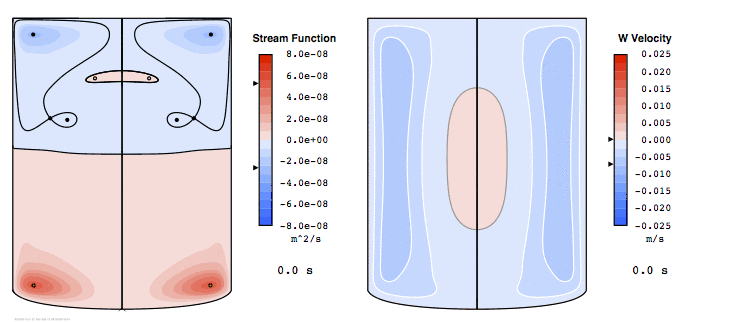
I will be analyzing this system in greater depth soon, focusing on compositional effects, meltback, and constitutional stability. This type of flow visualization will greatly help me make sense of the complex interactions of buoyancy and rotational forces in this system. It's going to be fun.