Implicit time integration methods in Cats2D

Cats2D Multiphysics > Research Topics > Implicit time integration methods in Cats2D

Implicit time integration methods in Cats2D

Comparing backward Euler to trapezoid rule

I have written some new notes that explain which time integration methods are used in Cats2D, and how these methods behave. This is a topic I never found time to write about in the user manual, so eventually this material will end up there. The notes are an outgrowth of my recent work on an oscillatory flow that emerges during time integration of a vertical Bridgman system. As part of that work I ran tests comparing the second-order trapezoid rule (TR) to the first-order backward Euler (BE) method. This got me interested in the second order backward difference formula (BDF2), a popular alternative to the trapezoid rule for solving stiff equations. So I installed it in the code and ran some tests on it too.

All three methods are A-stable, which is a must for this kind of work. But BE requires a much smaller time step than TR or BDF2 to achieve good accuracy on nontrivial problems, so it loses badly on efficiency. This is mostly because of the difference in convergence order of the methods, first versus second, but BE is also dissipative whereas TR is not. This gives BE the tendency to artificially attenuate oscillations, which could mask the presence of weak physical instability. BDF2 is also dissipative, but only slightly.

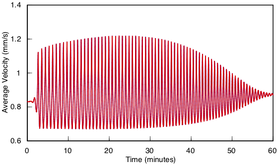
I show here computations of unstable natural convection that I've found in a vertical Bridgman system operated with a destablizing temperature profile. RMS average velocity is plotted versus time starting at the onset of growth from a steady, but unstable, flow computed with the growth interface held fixed. After a few minutes the instability sends the flow into a limit cycle. Initially the period is 53 seconds and gradually decreases to 41.5 seconds as the system stabilizes. Both curves were computed using TR, the blue curve with a step size of 0.25 seconds and the red curve with a step size of 0.10 seconds. The agreement is so close that the blue curve is hardly distinguishable under the red curve, indicating convergence of the TR method with respect to step size:

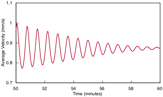
Examining the final minutes of unstable flow shows that the period has not drifted at all between the calculations:

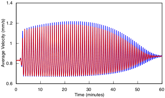
In this next comparison, the blue curve was computed by TR and the red curve by BE, using a step size of 0.25 seconds in both cases. The amplitude differs visibly throughout the integration, indicating that BE is far from convergence at this step size. The dissipative nature of BE is made apparent by its progressive tendency to underestimate the amplitude:

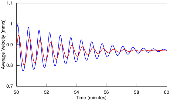
The error in period predicted by BE is not nearly as bad as amplitude, but it does drift somewhat from the TR result, as shown by this plot of the final ten minutes of decay:

Reducing the step size to 0.1 seconds for BE noticeably improves the situation, but some disagreement is still evident:

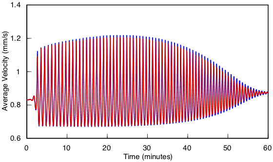
The drift in the period is only very slight, however, at this step size:

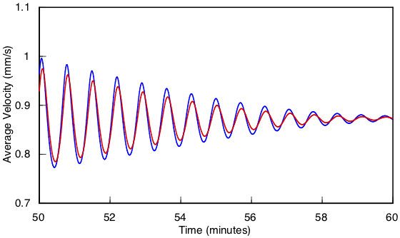
Reducing the step size to 0.025 seconds for BE achieves reasonable agreement with the TR results.

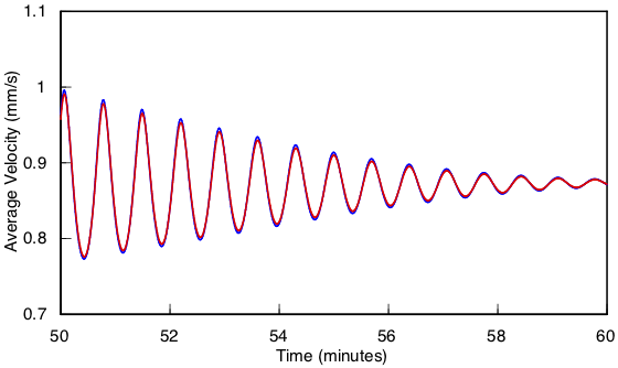
But the cost was very high. BE required ten times as many time steps as TR, and there was very little reduction in computational effort per time step to offset it.

These tests required over 300,000 time steps to complete. Was it worth it? You betcha. It gives me peace of mind to know that the limit cycle predictions shown here are robust to changes in numerical methods and parameters. Also, it is a good demonstration of the considerable advantage that TR has over BE in terms of accuracy and performance. Its non-dissipative character is particularly beneficial to the careful probing of weakly unstable flows, for example in the neighborhood of a bifurcation.

Comparing BDF2 to trapezoid rule

Next I show a comparison of TR to BDF2 on the same problem. First I computed solutions by the trapezoid rule at step sizes of 0.1 and 0.05 seconds, which I extrapolated to zero step size by Richardson extrapolation. The error is estimated from the difference between this extrapolated solution and a computed solution, which I show below for step size of 0.25 seconds (the blue curve) and 0.05 seconds (the red curve).

For convenience I have scaled the error by a flow magnitude of 1 mm/s. The time average of the actual magnitude is slightly smaller than this, around 0.9 mm/s, so the raw error is nearly equal to the percent relative error. The maximum value of the blue curve is 0.0072, about 0.8% relative error, and the maximum value of the red curve is 0.00027, about 0.03% relative error. The time steps differ by a factor of five, so the error should be 25 times smaller for the red curve, and these numbers bear this out, giving a ratio of 27.

This next plot shows how BDF2 (the blue curve) compares to the trapezoid rule (the red curve). A step size of 0.25 seconds was used in both cases:

The BDF2 error is four times larger, as predicted by theory. To achieve a comparable accuracy to TR it is necessary to halve the step size to 0.125 seconds for BDF2. When this is done the error is nearly identical, such that the blue curve cannot be seen beneath the red curve, at a cost of doubling the number of time steps.

In my work I want this kind of error to be small, no more than a percent or two. For this problem, the trapezoid rule with a step size of 0.25 seconds satisfies this desire. There isn't much value in reducing the error any further, so a smaller step size is overkill. Obviously there is not any advantage to using BDF2 for this problem, but I have found a completely different problem where BDF2 gives the correct outcome and TR does not. I will report on this later.