Cats2D Multiphysics > Research Topics > Computing mass transport in liquids

All unpublished results shown here are Copyright © 2016–2019 Andrew Yeckel, all rights reserved

Computing mass transport in liquids

I have collated some entries from my developments page into this article that discusses how accurate pathline integration can be used to study mass transport in liquids where small diffusion coefficients tend to make the problem very stiff.

Comparing the convective-diffusion model to the particle convection model

I'm intrigued by the possibility of using pathline integration to study strongly convected mass transport. The mixing studies I presented elsewhere correspond to a limiting case of mass Peclet number equal to infinity. In the absence of molecular diffusion there is no mass transport between neighboring points, so each point traced by the pathline integration maintains its original concentration. There is plenty of mixing so that points of low and high concentration are brought close together, but this mixing does not extend to length scales smaller than the thickness of the striated layers formed by convective transport along the streamlines of the flow. Furthermore, points within closed recirculations do not mix with points outside.

Unless these points are actual particles with properties distinct from the liquid, molecular diffusion will eventually cause these layers to mix. Yet convective flows often yield Peclet numbers greater than 10⁵ for transport of ordinary molecules in liquid, and 10⁸ or larger for macromolecules. We expect the limiting behavior of pathline transport without diffusion to accurately describe mixing over some initial period of time in such systems. Continuum mass transport at large Peclet numbers results both in stiff time integration requiring small time steps, and sharply defined spatial oscillations requiring a fine mesh. As these requirements can become prohibitive, it would be useful to know under what circumstances it is feasible to apply pathline integration in lieu of continuum modeling.

To study this issue I compare mixing computed by pathline integration to continuum mass transport computed from a convective-diffusion model. Mixing starts from a linear concentration distribution shown on the left below. The model flow, shown on the right, is a steady state Stokes flow driven by motion of the upper and lower surfaces in opposite directions. This flow features two co-rotating recirculations enclosed by a saddle streamline in the form of a figure eight or hourglass.

After 12.6 dimensionless time units, the continuum model with Peclet = 10⁵ shown below on the left strongly resembles pathline integration shown on the right. I've seeded paths at 291,384 node positions, compared to 56,481 concentration unknowns in the continuum model. Diffusion has reduced the difference between global maximum and minimum concentration by 5% compared to the starting concentration field. The pathline integration never reduces this measure because each point retains its initial concentration, and mixing only occurs at larger length scales by the formation of ever thinner spiral layers.

 

The next results show 31.4 time units of mixing. The maximum concentration difference has fallen by 10% in the continuum model. The spiral layers in concentration are somewhat less distinct in the continuum model. This is roughly the point at which I judge the models to start deviating significantly from each other.

The difference in models is much starker after 62.8 time units, shown next. The pathline integration exhibits a large number of spiral layers, but the continuum model shows only a small hint of them. The maximum concentration has fallen by 30%.

The dimensionless time is based on a characteristic time t* = L_o/U_o, where L_o is the cavity width and U_o is the velocity of the moving boundary. This is the transit time of the boundary, the time taken to move fluid from one side of the cavity to the other. In one of these transit times, fluid will move a quarter of a trip around the cavity, forming a quarter of a spiral layer of high and low concentration fluid. The number of spiral layers of high and low concentration created in time t is N = t/2t*. The rainbow color map used here makes it difficult to discern the actual number of layers, however, because the map introduces spurious color bands, mainly green and yellow, that do not represent maxima or mimima (ridges or valleys) in the concentration map. The situation is clearer when the warm-cold color scale is used, shown here after 12.6 and 31.4 time units of mixing.

The image on the left has 14 bands of high and low concentration spanning the cavity horizontally through each vortex center, thus 12 bands have been created in 12.6 time units. The image on the right has 30 new bands created in 31.4 time units. Agreement with the simple formula is excellent.

Initially the diffusion length is the entire span of the cavity and the rate of diffusion is small compared to convective mixing. After some number of spiral layers have been formed, the length scale over which concentration varies is small enough for diffusion to become comparatively large. We can estimate this crossover point by comparing the width of a layer, which is inversely proportional to the integration time, to the diffusion length, which is proportional to the square root of time:

The term in parentheses in the denominator is the rate at which concentration bands are created (two per spiral layer). Scaling the time by this rate gives the dimensionless form:

Rearranging gives us an estimate of the dimensionless integration time at which concentration variations diffuse away faster than bands are formed:

We expect that pathline integration will be a reasonable model of convective mass transport for integration times appreciably shorter than this criterion, which is 29 time units under the conditions of the simulation. In the pictures shown above, the spiral arms remain mostly recognizable after 31.4 time units, but have largely vanished after twice this long, 62.8 time units. The criterion gives sound guidance. The precise number is less important than the scaling in terms of Peclet number, which is a one third power. For each factor of ten increase in Peclet, the validity of pathline integration extends further in mixing time by approximately a factor of two (ten raised to the one third power).

I have tried computing the continuum model at Pe = 10⁶, but the mesh used here, 100x140 elements, fails to give a satisfactory result because of spurious spatial oscillations of concentration. I could probably capture the solution at this Peclet number reasonably well by doubling the mesh density, but things are getting expensive by then. Pathline integration makes a reasonable alternative for the first ten or so spiral arms formed at this Peclet number. These numbers suggest that we can reasonably begin to apply the zero diffusion limit around the same time we lose the ability to accurately resolve the continuum model at reasonable cost.

Mixing of two layers of liquid

Modeling segregation in melt crystal growth is difficult. Almost no one can do it well. Mass transfer is inherently time-dependent. Diffusion in liquids is always slow, so the equations are stiff in time and space, placing strict demands on element size and time step size. Failure to observe these demands often ends in numerical instability.

There are other challenges. In a moving boundary problem the domain itself is in motion, which raises important issues in how the differential equations and their discretization are cast. Cats2D uses an arbitrary Lagrangian-Eulerian (ALE) form of the equations that conserves mass and momentum accurately. Conservation boundary conditions also must be formulated carefully. Gross failure to conserve mass is likely to occur if these things are not done precisely.

I have run some tests on mass transport in an isothermal system in which flow is generated by a pumping motion of the baffle. The surface of the liquid rises and falls as the baffle is raised and lowered. The mesh elements expand and contract as well, so the computational domain is in motion relative to the laboratory reference frame. Many things can go wrong in a simulation like this, making it an excellent test of the code.

Below I show mixing of two layers of liquid initially having different concentrations of a fast diffusing molecule in water. The inner diameter is 2 cm and the total amount of liquid is 13.2 milliliters. The viscosity is 0.001 Pa-s. The diffusion coefficient is 10^-8 m²/s, two to three times faster than typical for small molecules. I used a high value to soften the numerics a bit. Even then the Peclet number equals 10000, indicating that mass transport is strongly convected under these conditions. In one case I've made the layers equal in volume, in the other case I've restricted the lower layer to the region under the baffle. The rate of motion in the animations is depicted in real time.

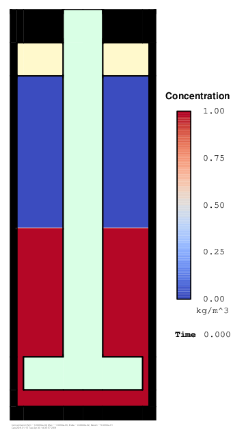
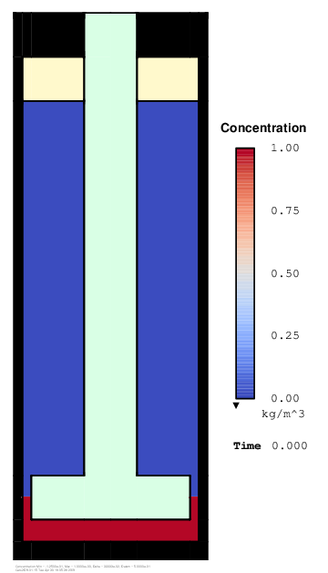
Inertia makes the flow highly irreversible. Wakes churn around the baffle with a salutary effect on mixing. The improvement is dramatic. The boundary between areas of high and low concentration stretches rapidly and spirals around itself, quickly reducing the mixing length to the diffusion length. Two strokes of the baffle are enough to mix the layers.

Conservation of mass is very accurate with total mass loss or gain less than 0.1% over the entire time integration. To achieve this I used a fine discretization with 332,391 unknowns. Variable time stepping with error control required approximately 1000 time steps per period at this Reynolds number. The wall clock time per time step on my modest laptop computer was about 10 seconds, so these animations took about 15 hours each to compute and draw the frames.

These computations allow very little compromise in numerics. A fine grid is required throughout the entire domain to capture the many sharp internal layers created by the swirling flow. Very small time steps and a high quality second-order time integrator are needed to conserve mass accurately (BDF2 was used in these computations). Numerical instability is difficult to avoid unless active time step error control is used. A robust linear equation solver is needed, and you'll be waiting around for a long time if it isn't very fast.

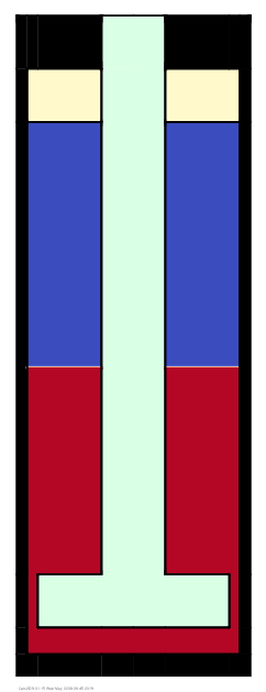
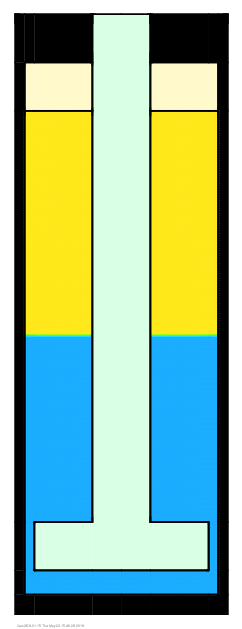
Let's compare the particle convection model to the convective-diffusion model. On the left is a frame from the convective-diffusion model. In the middle is a frame from the particle convection model. Red and blue particles turn into an swarming mess of purple in these visualizations, so on the right I have tried the Swedish flag colors for better contrast. I think I prefer it for the particle visualizations.

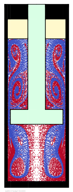
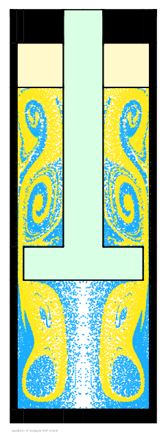
The agreement is remarkable. The particle convection model reproduces many fine details of the convective-diffusion model. This lends faith in both models, which are drastically different from one another, both in their mathematical formulations and in their algorithmic implementations. There are some issues with this comparison that are not obvious, but I will defer their discussion to the end of this post.

Mouse over the images below to see more broadly how the two models compare. After two strokes of the plunger the unmixed length scale has been reduced to the point that diffusion becomes important and the models substantially deviate from one another. In the early stages, however, when most of the mixing occurs, the particle convection model gives a very informative view of mass transport.

See both animations run simultaneously in a separate window (this might take a few moments to load).

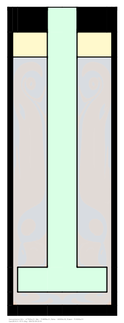
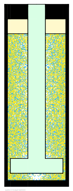
Diffusion has largely homogenized the two layers after five piston strokes (below left). Without diffusion the particles are fairly well mixed, but not perfectly so (below right).

It should be noted that the diffusion coefficient used here, D = 10^-8 m²/s, is three to ten times larger than typical of small molecules. A smaller more realistic value is very expensive and difficult to simulate because of the sharp concentration gradients found throughout the domain. These gradients place tight restrictions on time step and element size. In Cats2D all equations are solved simultaneously on the same mesh (no sub-gridding), so these restrictions carry over to the flow equations.

What else should we know?

If conditions are such that a particle convection model can be used to study convective mixing, it is necessary to solve only the flow equations. A factor of three reduction in CPU time is obtained by eliminating the species transport equation and its restrictions. There are fewer unknowns, a larger time step can be used, and the Jacobian is better conditioned which translates to a faster elimination by the frontal solver. The added effort needed to integrate the particle pathlines is modest. I was able to reduce the total number of elements by a factor of four without compromising the solution, which gained an additional factor of five speedup. Overall the CPU time needed to simulate one period of plunger motion was reduced from 3 hours to 12 minutes with these changes.

Now about those issues I alluded to earlier. The pathline integrations shown here have been seeded with approximately 20,000 fictitious particles uniformly spaced in the liquid. The particles represent mathematical points, but we must draw dots else we cannot see them. These dots will overlap in the drawing where two particles have approached close to one another. Consider what happens when uniformly spaced particles are subjected to an extensional flow. Spacing between the particles stretches in one direction and compresses in the other direction.

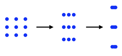
Empty space is created in the drawing when the dots overlap. The total areas of dots and empty space are not conserved, something I brought up earlier in the "Paint the sky with stars" entry half way down this page. This explains in part the appearance of white space in the particle visualizations when none was apparent in the initial condition. This is particularly obvious underneath the plunger at the start of the simulation where the flow is strongly extensional along the center axis.

However, there is more going on here than meets the eye. The equations represent conservation in a cylindrical geometry, but are visualized in a planar cross-section on the page. Areas near the center axis represent comparatively little volume. Quite a bit of plunger has been removed at the top of the stroke in terms of its planar cross-section, but most of it comes from the narrow shaft, so the volume removed is not so great as it appears. The liquid level falls only slightly to compensate for this small volume, far less than the area created underneath the plunger in the drawing.

As a consequence the total area of the liquid displayed in the drawing is larger at the top of the stroke than at the bottom, even though its volume remains constant in the problem formulation. For this reason alone empty space will increase when the plunger is withdrawn. But there is another important implication regarding the particles themselves. If we regard them as objects in the cylindrical geometry, they must represent toroids rather than spheres. To maintain a fixed volume, the cross-sectional area in the plane must increase when a particle moves towards the center axis. The concept is illustrated below using bagels.

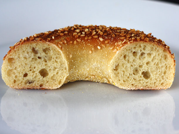
Obviously we aren't doing this with our dots of constant size. When particles rush under the plunger as it is withdrawn they fail to cover all the new area created there because they don't grow in size to satisfy conservation. This explains the growth and decline of empty space along the center axis as the plunger is raised up and down in the visualizations.

This isn't a problem per se, we just need to be aware of it and avoid drawing unwarranted conclusions about conservation of mass from these artifacts of the visualization. The only thing conserved is the number of particles, which have no volume. Their purpose is to provide a pointwise representation of the concentration field and they do so accurately at modest computational effort.